Lab 10
The purpose of this lab was to create a Bayes filter for the robot in the simulator to perform localization and predict the location of the robot in the map.
Bayes Filter
In the Bayes filter, we discretize our robot state into grid cells along the map. Our robot state is 3-D (x,y,\(\theta\)), where x is the x-coordinate of the robot in the map, y is the y-coordinate of the robot in the map, and \(\theta\) is the angle of the robot (where in this case, it is defined from -180 to 180 degrees, not 0 to 360 degrees).
The core idea of the Bayes filter is that we have a probability distribution over the grid of where we believe the robot can be. We have two steps to update the overall probability distribution. We first run the prediction step, where we predict where we think the robot will be based off of some control input and the prior belief. We then run the update step, where we modify our prediction and correct it based off of some sensor measurement. We do this by calculating the probability that our prediction is correct given that we received this sensor measurement.

Implementing the Bayes Filter
The main portion of this lab was getting the Bayes filter algorithms written. I mostly looked at TA Anya’s code for inspiration, but wrote up my understanding of the code below (and changed a few things to make things make more sense to me).
Compute Control
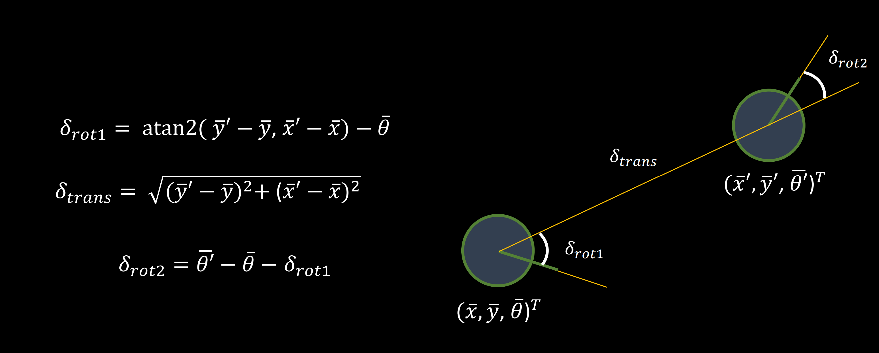
This is a helper function that will help us compute some control. In our Bayes filter, we need to have some sort of motion model, where we have some way of predicting our robot’s motion through some “control”. In our robot, we used the odometry motion model, in which we can predict our robot’s movement given we measure some rotation and translation of the robot in the global reference frame. However, this also works in reverse, where we can compute what the control inputs are required to move a robot from point A to point B (in this case, cell to cell), compare that to the actual measured control input, and use that to do the prediction step of our Bayes filter. Thus, compute_control calculates the values shown below using the equations shown below:

def compute_control(cur_pose, prev_pose):
    """ Given the current and previous odometry poses, this function extracts
    the control information based on the odometry motion model.

    Args:
        cur_pose  ([Pose]): Current Pose
        prev_pose ([Pose]): Previous Pose

    Returns:
        [delta_rot_1]: Rotation 1  (degrees)
        [delta_trans]: Translation (meters)
        [delta_rot_2]: Rotation 2  (degrees)
    """
    x_cur = cur_pose[0]; y_cur = cur_pose[1]; yaw_cur = cur_pose[2];
    x_prev = prev_pose[0]; y_prev = prev_pose[1]; yaw_prev = prev_pose[2];

    delta_rot_1 = np.degrees(np.arctan2((y_cur-y_prev),(x_cur-x_prev))) - yaw_prev
    delta_trans = np.sqrt((x_cur - x_prev)**2 + (y_cur - y_prev)**2)
    delta_rot_2 = yaw_cur - yaw_prev - delta_rot_1
    return delta_rot_1, delta_trans, delta_rot_2
Odometry Motion Model
This is another helper function gives us the probability that our robot moved from one location to another given the two locations and the actual control inputs (which are given to us). We will use the Gaussian in order to calculate this. The way that made sense to me is that we have the Gaussian centered around \(\mu = 0\) and we calcuate the value at \(u_actual - u_predicted\),using the compute_control function to find $$u_predicted4$ and with the covariances being given to us in BaseLocalization.
def odom_motion_model(cur_pose, prev_pose, u):
    """ Odometry Motion Model

    Args:
        cur_pose  ([Pose]): Current Pose
        prev_pose ([Pose]): Previous Pose
        (rot1, trans, rot2) (float, float, float): A tuple with control data in the format
                                                   format (rot1, trans, rot2) with units (degrees, meters, degrees)

    Returns:
        prob [float]: Probability p(x'|x, u)
    """
    u_pred = compute_control(cur_pose,prev_pose) #This is the u that should have gotten us to this location

    rot1_pred = mapper.normalize_angle(u_pred[0]); trans_pred = u_pred[1]; rot2_pred = mapper.normalize_angle(u_pred[2]);
    rot1 = mapper.normalize_angle(u[0]); trans = u[1]; rot2 = mapper.normalize_angle(u[2]);

    prob_rot1 = loc.gaussian(mapper.normalize_angle(rot1_pred - rot1),0,loc.odom_rot_sigma)
    prob_trans = loc.gaussian(trans_pred - trans, 0, loc.odom_trans_sigma)
    prob_rot2 = loc.gaussian(mapper.normalize_angle(rot2_pred - rot2),0,loc.odom_rot_sigma)

    prob = prob_rot1 * prob_trans * prob_rot2

    return prob
Prediction Step
This is the function to perform the prediction step. We use the nested for-loops to iterate through every grid cell twice. We compare each grid cell to every other grid cell (this is a little bit redundant, but I can’t get it to work otherwise cause 3-D matrices hurt my brain and Python for-loops suck) and update each one with the probability that one could move to the other given the odometry information. I don’t believe we have to normalize it here as long as we normalize it at the end, but Anya did so I kept it in there.
def prediction_step(cur_odom, prev_odom):
    """ Prediction step of the Bayes Filter.
    Update the probabilities in loc.bel_bar based on loc.bel from the previous time step and the odometry motion model.

    Args:
        cur_odom  ([Pose]): Current Pose
        prev_odom ([Pose]): Previous Pose
    """

    u = compute_control( cur_odom, prev_odom )

    # Initialize bel_bar to 0
    temp = np.zeros((12, 9, 18))

    for cx_prev in range(12):
        for cy_prev in range(9):
            for ca_prev in range(18):
                if (loc.bel[cx_prev, cy_prev, ca_prev] > 0.0001):
                    for cx_cur in range(12):
                        for cy_cur in range(9):
                            for ca_cur in range(18):
                                #Obtain the center coordinates of each grid cell
                                cur_pose = mapper.from_map(cx_cur, cy_cur, ca_cur)
                                prev_pose = mapper.from_map(cx_prev, cy_prev, ca_prev)

                                #Compute the probability that we're in the cell given some control input and some previous pose
                                p = odom_motion_model(cur_pose, prev_pose, u)

                                #Obtain the previous belief of that cell
                                bel = loc.bel[cx_prev, cy_prev, ca_prev]

                                #Update the grid cell
                                temp[cx_cur, cy_cur, ca_cur] += (p * bel)

    norm_factor = np.sum(temp)
    loc.bel_bar = np.true_divide(temp, norm_factor)
Sensor Model
Like we compute the probability that our robot moved somewhere based on the controls (or that the controls led the robot there), we also want the probability that we are in a given location given our sensor measurements. We do this by comparing our measured sensor measurements to the predicted sensor measurements, which are given to us. We model our sensor with a Gaussian, similar to our odometry motion model. I once again used a Gaussian centered at 0 and calculated it at \(z_actual - z_predicted\), using the sigmas given to us in the BaseLocalization class. Because I know that our robot collects 18 values, I can use the hard-coded value of 18 to initialize my probability array and iterate through the for loop like that.
def sensor_model(obs):
    """ This is the equivalent of p(z|x).


    Args:
        obs ([ndarray]): A 1D array consisting of the true observations for a specific robot pose in the map

    Returns:
        [ndarray]: Returns a 1D array of size 18 (=loc.OBS_PER_CELL) with the likelihoods of each individual sensor measurement
    """
    prob_array = np.zeros(18);

    for x in range(0,18):
        prob_array[x] = loc.gaussian(loc.obs_range_data[x] - obs[x],0, loc.sensor_sigma)
    return prob_array
Update Step
In this function, we perform the update step on our grid. We iterate through the grid and update each cell by multiplying the belief bar (which is our intermediate belief based solely on our prediction step) by the probability that our sensor measurements are correct (or that we are actually in that grid cell based on our sensor measurements). Because we assume each sensor measurement is independent, we can just multiply our 18 individual probabilities to get one scalar value, and we use that joint probability to update each cell. Here, the normalization step is necessary (to turn it back into a probability distribution).
def update_step():
    """ Update step of the Bayes Filter.
    Update the probabilities in loc.bel based on loc.bel_bar and the sensor model.
    """
    for cx_cur in range(12):
        for cy_cur in range(9):
            for ca_cur in range(18):
                #Get the current bel_bar of the current grid cell
                bel_bar = loc.bel_bar[cx_cur, cy_cur, ca_cur]


                p = sensor_model(mapper.get_views(cx_cur, cy_cur, ca_cur))

                #Because we assume all sensor readings are independent of each other, we can multiply the values together
                p_mul = np.prod(p)

                loc.bel[cx_cur, cy_cur, ca_cur] = p_mul * bel_bar

    # Normalize
    sum_val = np.sum(loc.bel)
    loc.bel = np.true_divide(loc.bel, sum_val)
Running the Bayes Filter
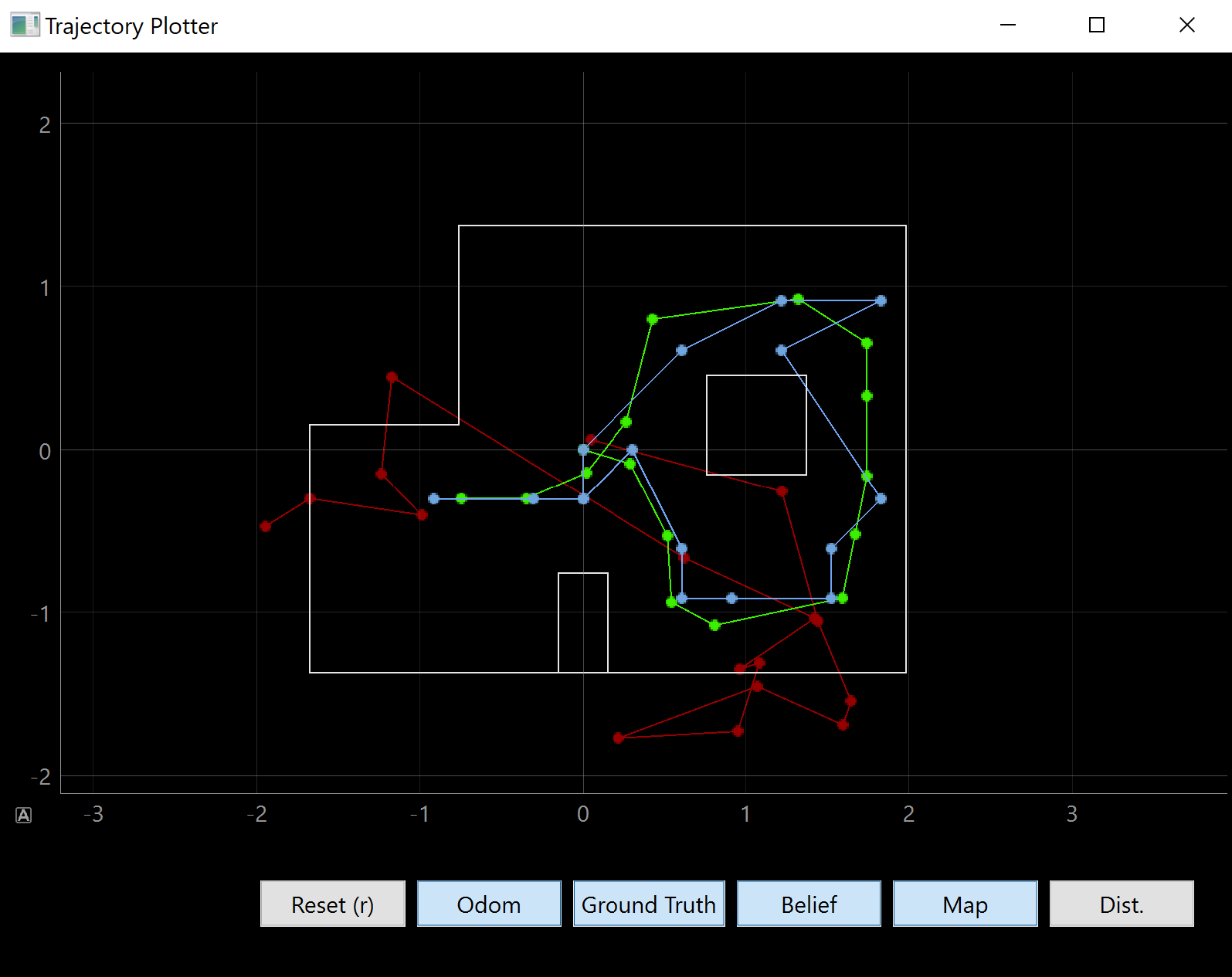
After I wrote all the helper functions, I ran the Bayes filter in the simulator to test if it worked and it worked surprisingly well. The odometry only (red) is meant to be trash since our robot’s accelerometer is not very good. However, as we can see, the blue (Bayes filter) seems to match the true pose of the robot (green) pretty well. It’s important to note that because we discretize our robot’s location, we must choose a spot within our cell to pick as our robot’s pose. As we can see, the classes pick the center of each grid cell.
