Lab 3
The purpose of this lab was to get the time-of-flight (ToF) sensors working and reading distances from them. We also used Bluetooth to send back data from the time-of-flight sensors.
Communicating with the ToF sensors
Each ToF sensor communicates utilizing the I2C protocol, which means that each sensor should have a unique I2C address. Unfortunately for us, each sensor comes hard-coded with the same I2C address (0x52), that means that we cannot communicate with both sensors as they’re given.
The two ways to get around this are 1) power off one sensor and change the I2C address of the other and 2) power one off and read the other, alternating so that you can read each sensor one at a time.
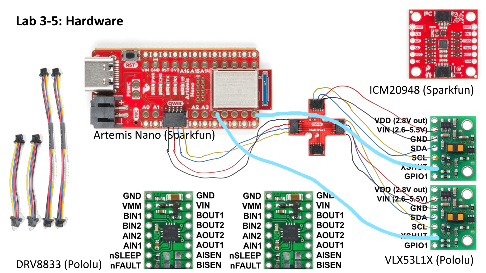
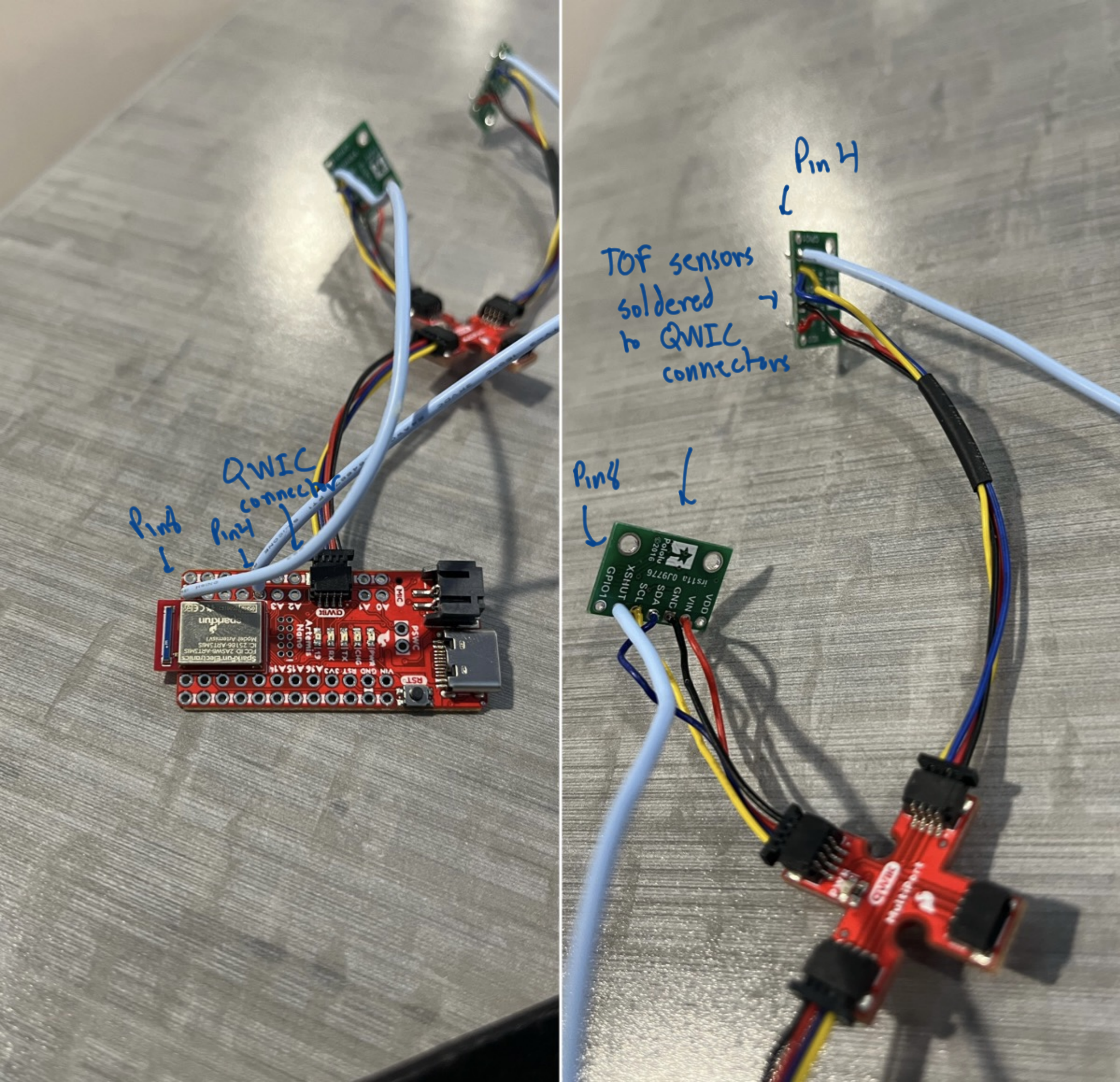
The way I chose to approach it was to turn off one of the sensors using the XSHUT pin and then re-write the I2C address of the other sensor. While this method only requires one of the sensors to have a wire soldered to their XSHUT pin, I have both sensors’ XSHUT pins soldered to a pin on the Artemis (mainly for troubleshooting). The main advantage to this strategy is that it is simpler to do, as you don’t have to code in additional logic to turn off one sensor at a time. You are also able to read data quicker, as each sensor has a boot-up sequence when you power it on. The main disadvantage to this strategy is that each sensor cannot remember when you rewrite their I2C address so you have to rewrite it everytime you power the sensor on. Another disadvantage is that you would always have both sensors on to avoid this issue, thus drawing more power.
The other method’s advantage is that you could potentially save power by only having the necessary sensors on when you need them. The disadvantage is that it’s more logically challenging to code and wouldn’t be able to collect data as quick as you have to wait for each sensor to power on, which could take time.
Sensor Placement
I chose to place two ToF sensors on my robot, with one facing forwards on the front of the robot and one facing left 90 degrees on the side of the robot. I chose these two positions because it makes calculating coordinates in relation to my robot’s reference frame easier and it’s easy to visualize what the robot should be seeing. However, this creates some pretty large blindspots, namely on the entire right-side of the robot, behind my robot, as well as a small area inbetween the two sensors. Therefore, my robot won’t be able to detect obstacles on those sides of the robot and will just crash. For instance, my robot could drift left, exposing its right side and crash that way. It could also back up into obstacles.
Wiring Diagram
Wiring Photos
Scanning for I2C Address
The Sparkfun people fortunately made many examples for the Artemis Nano, including one that utilizes the Arduino Wire.h library to communicate with I2C devices. We used this example (Example5_WireI2C) in order to scan the peripheral for I2C devices and return the I2C address of the device (in this case, the ToF sensor)
 As we can see, the program scans an extra port (that doesn’t seem to exist most likely just a Windows 10 thing) but it still can detect a device with an I2C address of 0x29. Now, this is the ToF sensor even though it doesn’t match the hard-coded 0x52. I’ve written both I2C addresses below in binary:
0x52 = 0b1010010
0x29 = 0b101001
It appears that the program bitshifts the I2C address it reads to the right one in order to remove the R/W bit of the I2C address so it displays 0x52 » 1, which is 0x29.
Testing 1 ToF Sensor
The ToF sensor has 3 distance modes: Short, Medium and Long. The advantages of using a shorter distance mode is that it is more accurate regardless of the lighting (since it limits the range to around 1.2 m), while the big disadvantage obviously being that it cannot see as far. For my robot, I decided that I would use the Long mode because I wasn’t sure what environments I would eventually be testing my robot in and might have to detect longer distances, especially if mapping eventually. However, if I’m just calibrating some other part of the robot and need the ToF data, then Short mode could be okay too.
Sparkfun provides a library for the VL53L1X distance sensor. In order to test the functionality of a single sensor, I used the provided example (Example1_ReadDistance), with the sensor set to long mode. I tested the range by walking around with the distance sensor and found that the range was ~4 m, which is honestly pretty long. In order to test accuracy, reliability, and ranging time, I took 64 measurements from 10 cm to 30 cm in 5 cm increments and then calculated the mean and standard deviation in order to compare to the true distance. I also measured the ranging time using the micros() function in Arduino.
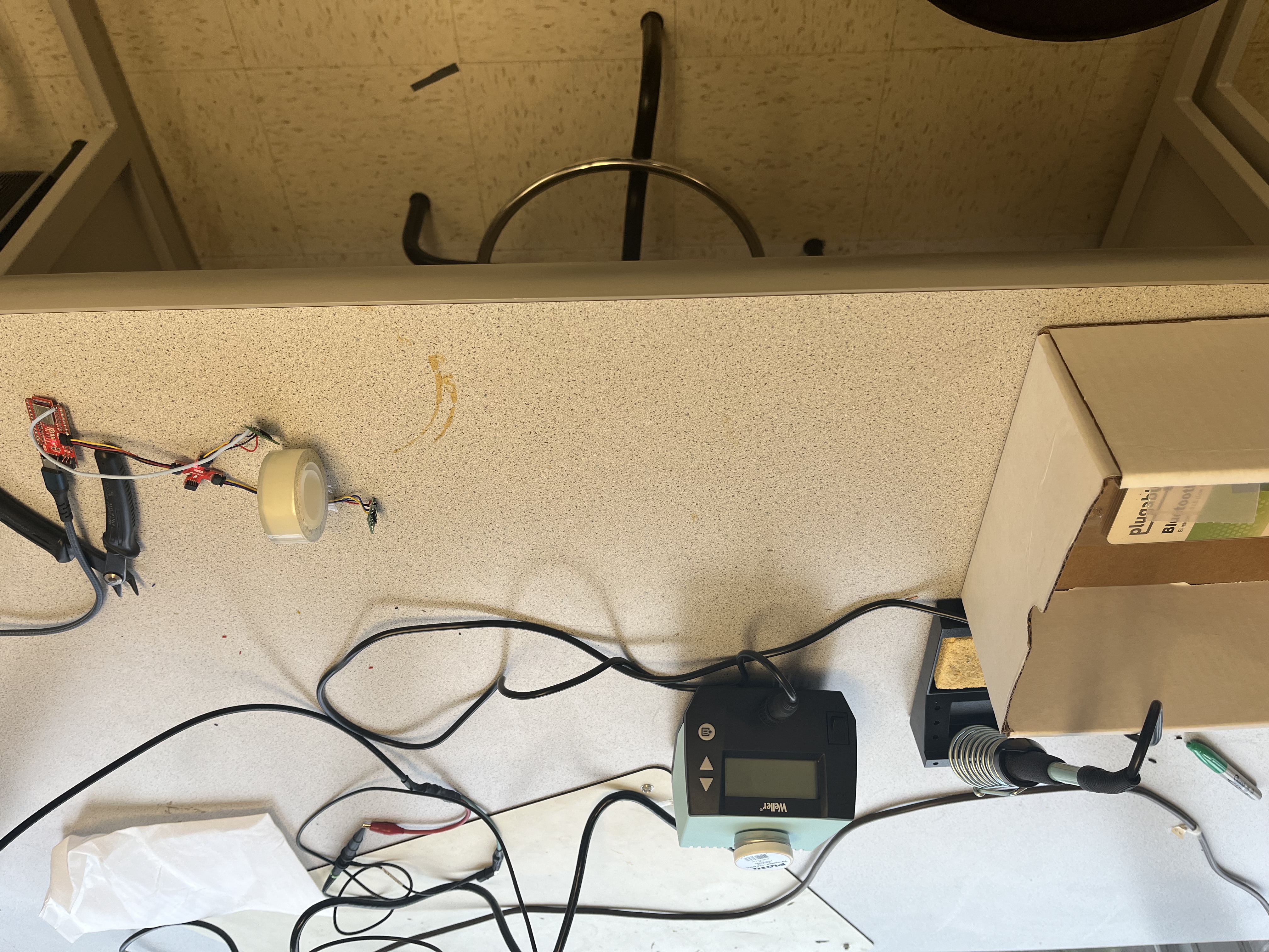
Photo of my setup:
 Here is a plot showing that below (the error bars are there, just very teeny which is a good thing I suppose):
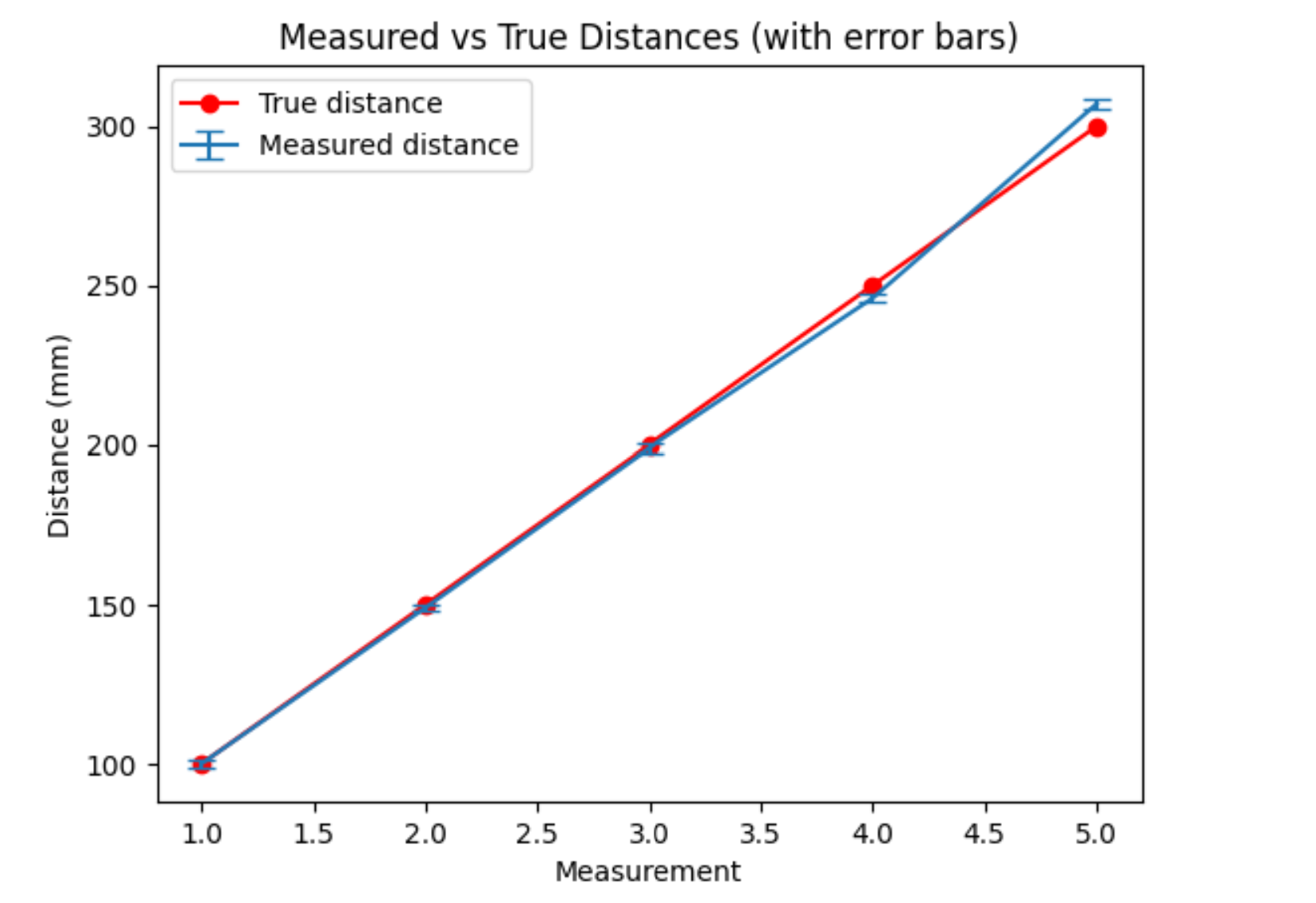
And the Python scripting code:
td = [100, 150, 200, 250, 300]
md = [100, 149, 199, 246, 307]
std = [1.25, 1.19, 1.34, 1.42, 1.55]
x = [1, 2, 3, 4, 5]
plt.plot(x,td,'r-o', label = 'True distance')
plt.errorbar(x, md, yerr = std, capsize = 5, label = 'Measured distance')
plt.legend()
plt.ylabel('Distance (mm)')
plt.xlabel('Measurement')
plt.title('Measured vs True Distances (with error bars)')
Ranging Time Table:
| Times | Ranging Time |
|---|---|
| With everything | 2.369 ms |
| W/o stopRanging() | 1.71 ms |
| Just reading | 1.056 ms |
And the Arduino code I used to measure it (the loop after all initialization steps):
void loop(void) {
  int times_sum = 0; int distance_sum = 0;
  int distances[64];

  for(int i = 0; i < 64; i++){
    distanceSensor1.setDistanceModeLong();
    distanceSensor1.startRanging();  //Write configuration bytes to initiate measurement
    while (!distanceSensor1.checkForDataReady()) {
      delay(1);
    }
    long t1 = micros();
    int distance = distanceSensor1.getDistance();  //Get the result of the measurement from the sensor
    //distanceSensor1.clearInterrupt();
    //distanceSensor1.stopRanging();

    long t2 = micros();
    distances[i] = distance;
    Serial.print("Distance(mm): ");
    Serial.print(distance);
    Serial.printf("   Time for ranging: %d", (t2-t1));
    times_sum = times_sum + (t2 - t1);
    distance_sum = distance_sum + distance;

    Serial.println();
  }
  long time_avg = times_sum/64;
  int distance_avg = distance_sum >> 6;
  int std = 0;
  for(int i = 0; i < 64; i++){
    int diff = pow(distances[i] - distance_avg, 2);
    std = std + diff;
    Serial.printf("Difference: %d \n", diff);
  }


  Serial.printf("Average ranging time: %d\n", time_avg);
  Serial.printf("Average distance: %d\n", distance_avg);
  Serial.printf("StDev value: %d\n", std);
  delay(5000);
}
Note that I had to calculate the standard deviation off board, since I couldn’t figure out sqrt() in Arduino, so the value I read isn’t actually the true standard deviation, just part of the calculation
Using 2 ToF Sensors
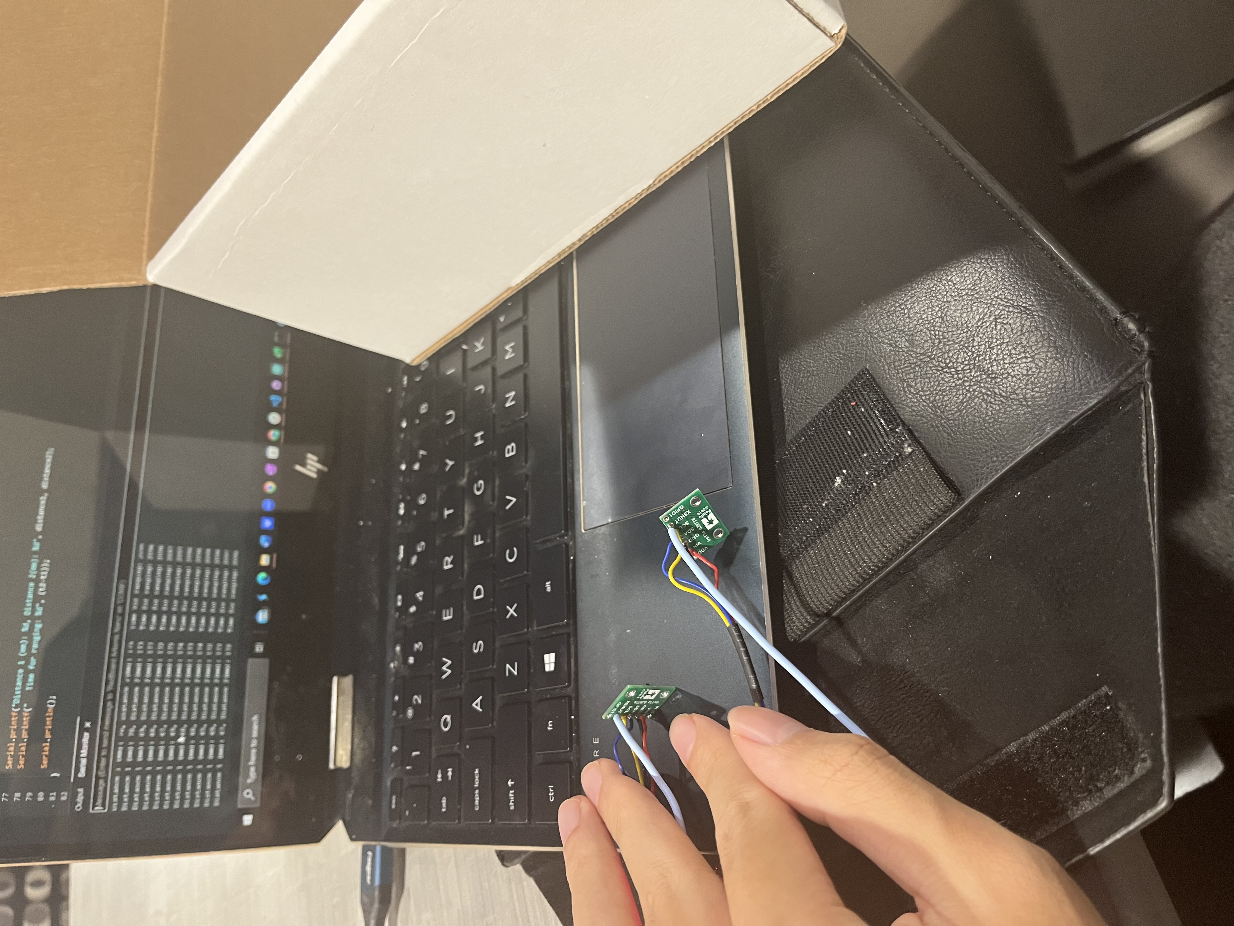
I used the rewrite I2C address method in order to read both sensors at the same time. Note that I had to connect to each sensor individually when using .begin() to initalize each sensor.
A photo of my setup:
Arduino code:
#include <Wire.h>
#include "SparkFun_VL53L1X.h"  //Click here to get the library: http://librarymanager/All#SparkFun_VL53L1X
#include <math.h>

#define XSHUT_PIN 8
#define XSHUT_PIN1 4
SFEVL53L1X distanceSensor1;
SFEVL53L1X distanceSensor2;


void setup(void) {
  Wire.begin();

  Serial.begin(115200);
  pinMode(XSHUT_PIN, OUTPUT);
  pinMode(XSHUT_PIN1, OUTPUT);

  digitalWrite(XSHUT_PIN, LOW);
  digitalWrite(XSHUT_PIN1, HIGH);

  if (distanceSensor1.begin() != 0)  //Begin returns 0 on a good init
  {
    Serial.println("Sensor1 failed to begin. Please check wiring. Freezing...");
    while (1)
      ;
  }
  distanceSensor1.setI2CAddress(0x25);
  digitalWrite(XSHUT_PIN, HIGH);

  if (distanceSensor2.begin() != 0)  //Begin returns 0 on a good init
  {
    Serial.println("Sensor2 failed to begin. Please check wiring. Freezing...");
    while (1)
      ;
  }

  Serial.println("Sensors online!");
  Serial.println(distanceSensor1.getI2CAddress());
  Serial.println(distanceSensor2.getI2CAddress());

  distanceSensor1.setDistanceModeLong();
  distanceSensor2.setDistanceModeLong();
}

void loop(void) {
  distanceSensor1.startRanging();  //Write configuration bytes to initiate measurement
  distanceSensor2.startRanging();

  while (!distanceSensor1.checkForDataReady() || !distanceSensor2.checkForDataReady()) {
    delay(1);
  }
 long t1 = micros();
 int distance1 = distanceSensor1.getDistance();  //Get the result of the measurement from the sensor
 //distanceSensor1.clearInterrupt();
 //distanceSensor1.stopRanging();
  int distance2 = distanceSensor2.getDistance();
  //distanceSensor2.clearInterrupt();
  //distanceSensor2.stopRanging();

  long t2 = micros();

  Serial.printf("Distance 1 (mm): %d, Distance 2(mm): %d", distance1, distance2);
  Serial.printf("   Time for ranging: %d", (t2-t1));

  Serial.println();
}
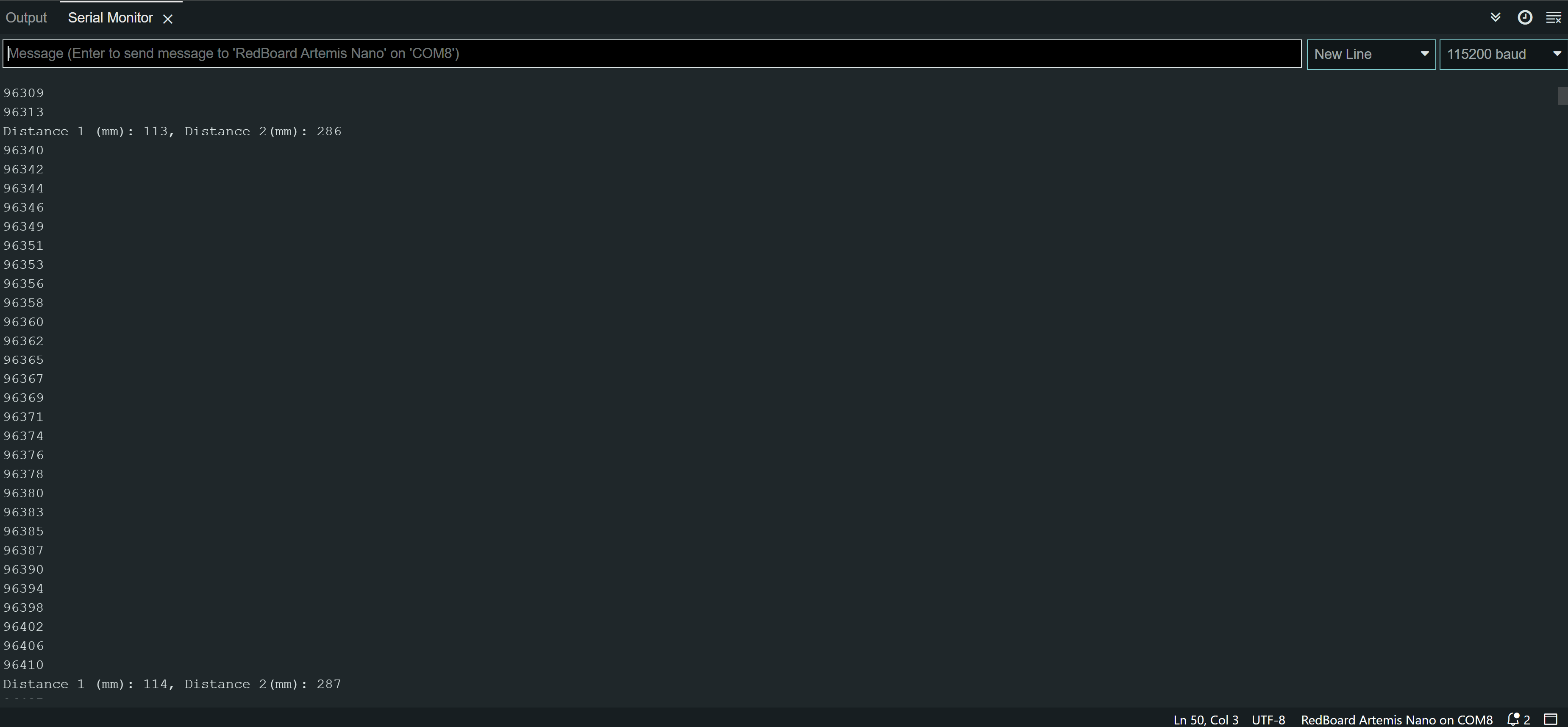
Serial output of my readings:

ToF Limiting Factor
In order to find out what the limiting factor was when measuring, I added a print statement that prints micros()/1000 (so we can easily see the ms) while the data isn’t ready, then prints the data once the data is ready (this is using the .checkForDataReady() function).
Arduino code snippet (exact same as above except I changed what is run within the while loop):
while (!distanceSensor1.checkForDataReady() || !distanceSensor2.checkForDataReady()) {
    Serial.println(micros()/1000);
  }
And the Serial output:
 ;
;
As we can see from the Serial monitor, it takes about 27 ms from when it prints the distance measurements to start printing time again, which means the reading of the data, the printing of the data, and running .startRanging() all take about 27 ms (note that this is without clearInterrupt() and stopRanging()). However, we are stuck in that while loop for about 70 ms which means it takes ~ 70 ms for the data to actually be ready. This means that the limiting step is the actual reading of the distance (and I have it on a pretty short distance too).
Collecting data over Bluetooth
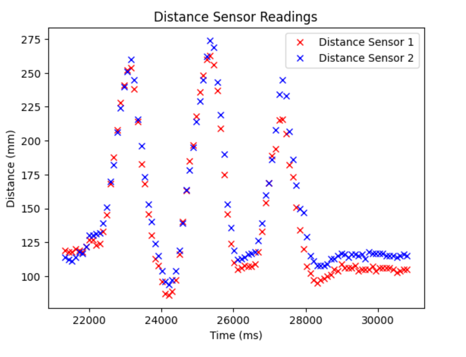
In order to collect data from the distance sensors over Bluetooth, I had to modify the Python files as well as the ble_arduino.ino file. I decided to collect 100 distance measurements along with their timestamps, measure the time elapsed, and then send them all back to be processed by a notification handler. I then extracted the timestamps, the distances, and plotted distance over time using matplotlib. I decided to use 100 distance measurements because then I could have a fixed array size, which would then allow me to iterate through it without going out-of-bounds (which is huge no-no for any microcontroller). All of the variables I used are global variables initialized outside of the case.
Arduino code (only the function to read values and write it back):
case GET_DIST:
          distanceSensor1.setDistanceModeLong();
          distanceSensor2.setDistanceModeLong();
          start_time = millis()/1000;
          for(int i = 0; i < size; i++){
            distanceSensor1.startRanging();  //Write configuration bytes to initiate measurement
            distanceSensor2.startRanging();

            while (!distanceSensor1.checkForDataReady() || !distanceSensor2.checkForDataReady()) {
              delay(1);
            }
            t[i] = float(millis());

            distance1 = distanceSensor1.getDistance();  //Get the result of the measurement from the sensor
            //distanceSensor1.clearInterrupt();
            //distanceSensor1.stopRanging();
            d1s[i] = distance1;
            distance2 = distanceSensor2.getDistance();
            //distanceSensor2.clearInterrupt();
            //distanceSensor2.stopRanging();
            d2s[i] = distance2;
          }
          stop_time = millis()/1000;
          Serial.printf("Time elapsed: %d seconds\n", stop_time - start_time);

          x = 0; y = 5;
          while(y <= size){
            tx_estring_value.clear();
            for(int i  = x; i < y; i++){
              tx_estring_value.append("T:");
              tx_estring_value.append(t[i]);
              tx_estring_value.append("|D1:");
              tx_estring_value.append(d1s[i]);
              tx_estring_value.append("|D2:");
              tx_estring_value.append(d2s[i]);
              tx_estring_value.append("|");
            }
            tx_characteristic_string.writeValue(tx_estring_value.c_str());
            Serial.println(tx_estring_value.c_str());
            x = x + 5;
            y = y + 5;
          }
          Serial.printf("Distance 1 (mm): %d, Distance 2(mm): %d", distance1, distance2);
          Serial.println();

          break;
Python code (notification handler and plotting code):
times = []
d1 = []
d2 = []
global times
global d1
global d2

def extract_distances(uuid, data):
    temps = ble.bytearray_to_string(data);
    temps = temps.split("|");
    temps.pop();
    for i in temps:
        if(i[0] == "T"):
            times.append(float(i[2:]));

        if(i[0] == "D" and i[1] == "1"):
            d1.append(float(i[3:]));

        if(i[0] == "D" and i[1] == "2"):
            d2.append(float(i[3:]));

ble.start_notify(ble.uuid['RX_STRING'], extract_distances)
ble.send_command(CMD.GET_DIST, "")

time.sleep(15);

ble.stop_notify(ble.uuid['RX_STRING'])
plt.plot(times, d1, 'rx', label = 'Distance Sensor 1')
plt.plot(times, d2, 'bx', label = "Distance Sensor 2")
plt.title('Distance Sensor Readings')
plt.xlabel('Time (ms)')
plt.ylabel('Distance (mm)')
plt.legend()
plt.show()
And the plot:
MEng Task 1
One type of IR distance sensor is an amplitude-based IR sensor. This one is one of the simpler ones, which simply emits an IR beam and then uses a photodiode in order to measure the strength of the IR beam that is reflected (more light means more voltage means closer). These tend to be used as proximity sensors/motion detection, but do work as short-range distance sensors. The pros of this type of sensor is that it’s very simple (photodiode + LED) and thus, very cheap. The cons are that it has a very short range and is very affected by the environment. Different materials absorb/reflect the outputted light differently and ambient light can saturate the photodiode, thus messing with the sensor readings.
Another type of IR distance sensor is the triangulation-based IR distance sensor. This one also emits an infrared signal, but measures the angle of the reflected signal using a position-sensitive photodetector. Thus, it uses math to detect the distance of the signal. The pro’s of this one is that it’s still relatively cheap compared to other options and has more range than the amplitude-based IR sensor. It is also less sensitive to the ambient environment and has greater range than the amplitude based one. However, it still doesn’t have great range (though this depends on the sensor) and is still affected by the ambient environment.
A third type of IR distance sensor is the one that we use, the time-of-flight distance sensor. This one shoots out an IR beam and measures the time it takes for the beam to return. The pros of this one is that it is the least sensitive to the ambient environment and has the greatest range and accuracy out of the three, and can get very quick measurements. The cons are that the time-of-flight sensor is the most complex and thus, tends to be more expensive than the other ones. It also is a lot more complex and processing the data can provide challenges sometimes.
MEng Task 2
I tested the ToF sensors on a variety of different textures, colors, and in light/darkness.
Photo of my setup:
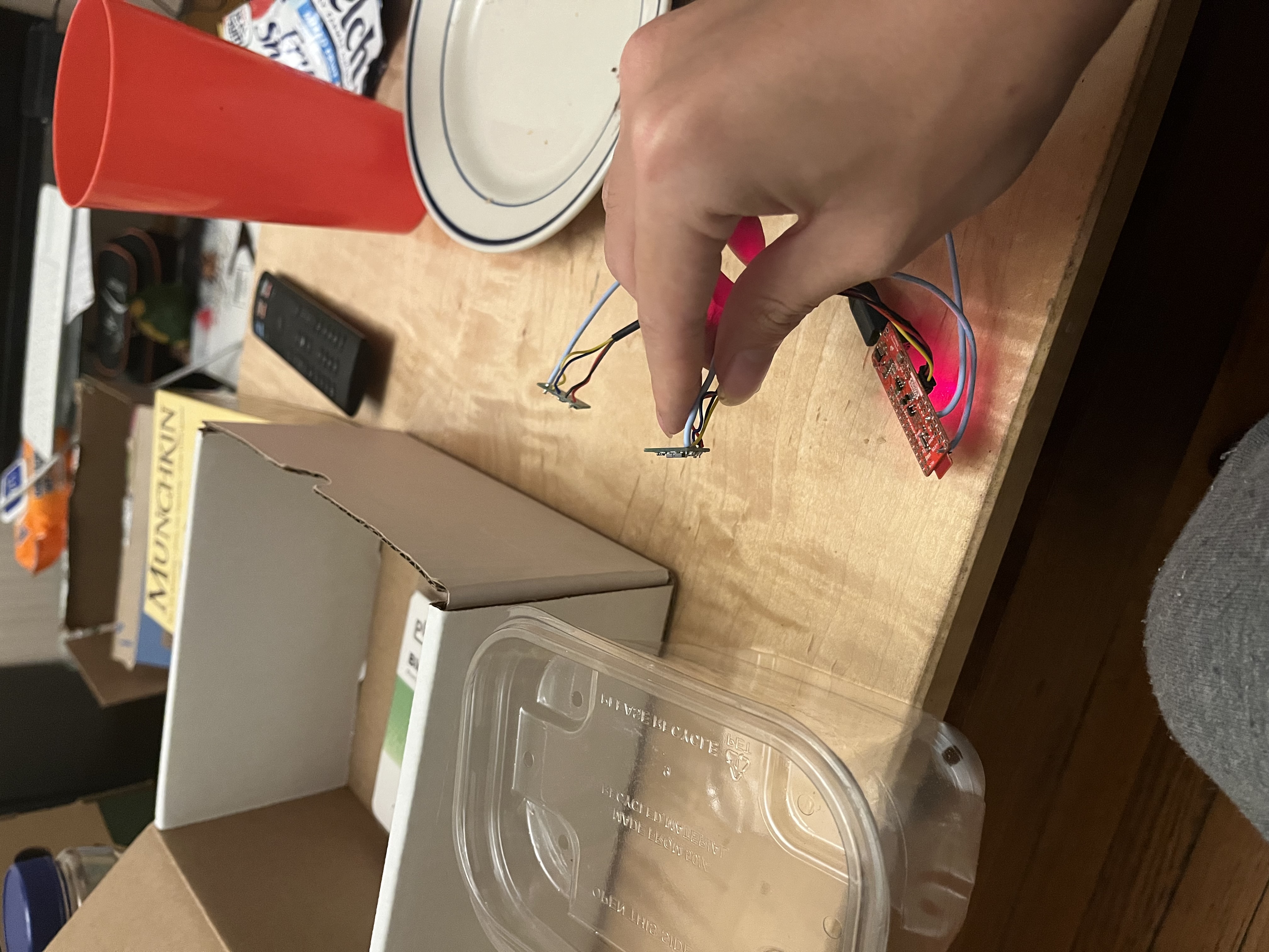 I got that the color didn’t really affect my readings in a noticeable (red, blue, black, white, and beige), nor did any of the textures I tested (couch, wall, blanket, wood). There was also no significant difference in darkness and light. The only surface that I noticed would mess with my sensors is when I aimed at a clear plastic container. The true distance was 80 mm and I was getting readings of around 124 mm with a standard deviation of ~ 5.5 mm, which is a lot higher than what it was when I tested the reliability (on a white cardboard box). I also noticed that it would read the surface of my laptop screen incorrectly, with the true distance being 100 mm and it returning values of ~170 mm, though the standard deviation was back to around 1.5 mm. This was mainly when the laptop screen was on.