Lab 7
The purpose of this lab was to figure out a way to estimate the location of the robot in between ToF sensor readings. This is because our ToF sensor readings are too slow and our system won’t be able to drive as fast. The best way to do this is with a Kalman filter, which we calculated and tested. However, I ended up implementing a linear extrapolator on the robot because it is simpler and more versatile with different battery levels.
Estimating drag and momentum
In order to do the Kalman filter, we need to estimate the dynamics of our system/state. Our state is defined as the distance from the wall and the velocity of our robot. Thus, we can estimate both using drag and momentum equations. Our state is thus defined as:
\[\begin{bmatrix} \dot{x} \\\ \ddot{x} \end{bmatrix} = \begin{bmatrix} 0 & 1 \\\ 0 & -d/m \end{bmatrix} * \begin{bmatrix} x \\\ \dot{x} \end{bmatrix} + \begin{bmatrix} 0 \\\ 1/m \end{bmatrix} * u\]In order to find the constants d and m, we needed to apply a step response to our robot and measure both the steady-state velocity and the 90% rise time (which is 0.9 times the time it took to reach that steady-state velocity)
In my code, I kept the car still for 3 seconds, then drove it at a wall using a PWM value of 85 (which is around the ) until it reached a steady velocity, all while measuring the ToF values. Here is the data for that:
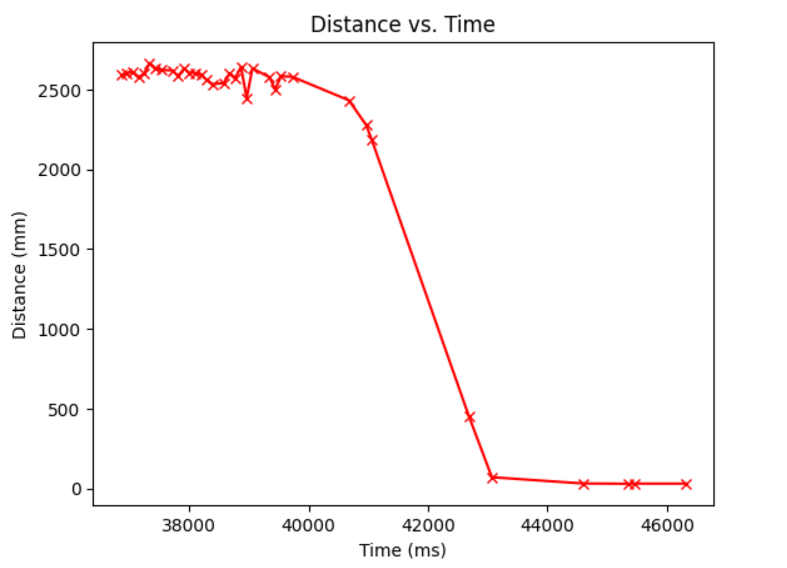
From this, I extracted the velocities using the differences between the distances divided by the time step. The graph looks a little funky because of the noise (a little different sensor measurements over a short time):
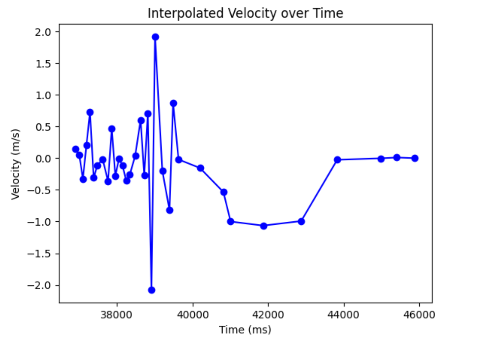
Looking at the time when the robot starts to move, it looks like this:
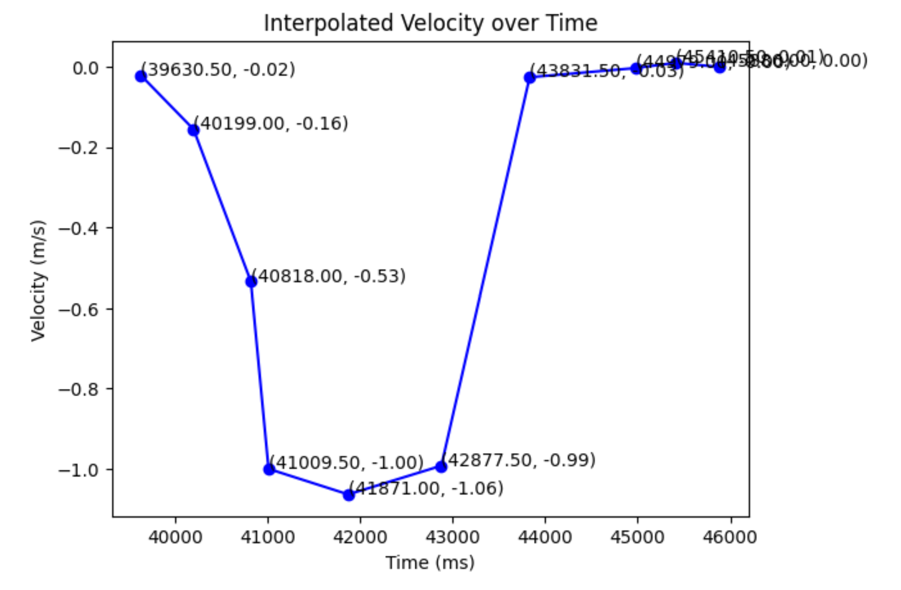
As we can see, the steady state velocity evens out around 1000 mm/s. This means that is our steady-state velocity, and we can calculate our drag term to be u/velocity, or 1/1000 mm/s. This means that when we input a u (control) into our Kalman filter, we will need to divide it by 85 because that’s the step response I used to calculate it.
I also looked at the graph to calculate the 90% rise time, which calculated by doing the equation: \(0.9t = (41009.5 - 39630.5) * 0.9 / 1000\) and got 1.2411 seconds.
I then calculated the m term, which was \((-d * t_{0.9})/(ln(0.1)) = 5.390 * 10^{-4}\)
With this, I finally had my A and B matrices. I set the C matrix to be \(\begin{bmatrix} -1 & 0\end{bmatrix}\) because we are converting our measurement (which is a positive measurement) into a negative distance measurement, which directly correlates to our state. The C matrix essentially describes how our measurement correlates to our state. The 0 represents the fact that we can’t measure the velocity of our robot.
Other Kalman filter parameters
The only other Kalman filter parameters that we need are the noise parameters. We have process noise and measurement noise.
\[{\Sigma}_u = \begin{bmatrix} ({\sigma}_1)^2 & 0 \\\ 0 & ({\sigma}_2)^2 \end{bmatrix}\] \[{\Sigma}_z = ({\sigma}_3)^2\]Our process noise describes the noise in our estimate of our state. As this can’t really be measured due to a myriad of factors, I estimated both parameters to be 10. With the sensor noise, we can measure the noise. I took a bunch of still-sensor measurements, calculated the standard deviation, and found it to be ~ 30 mm.
Offboard Kalman Filter
After I got all the parameters for the Kalman Filter, I tested it on some data that I saved from running the PI controller. Note that I had to discretize the A and B matrices because both were time dependent. This was mainly just multiplying them by the time elapsed.
Code to do this:
Below is a prediction with the aforementioned sigmas:
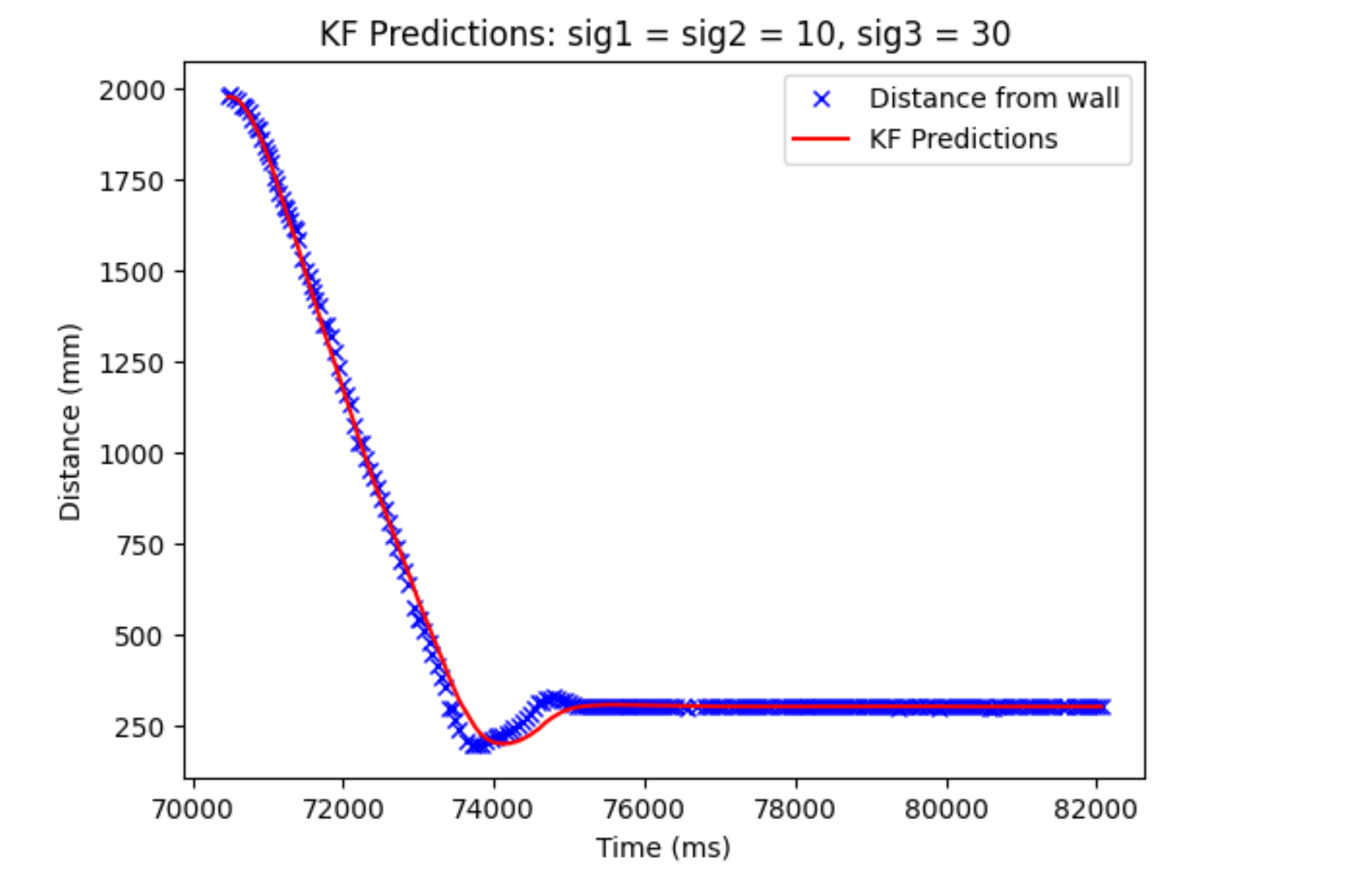
They might look different and the Kalman filter may look less accurate, but there is actually no telling which one is more accurate. We used to be measuring our distance from the wall with the ToF sensor and it is noisy and can be a little less accurate. Thus, it’s possible that our Kalman filter is actually more accurate at predicting how far our robot is from the wall and we should trust that more than just our sensor readings.
I also wanted to prove that I had everything working and it wasn’t just me reading my sensor measurements (which would work in this case, as the sensor measurements also happen to measure our state). Thus, I adjusted my parameters so my measurement noise was 3000, which would make it so that our Kalman filter only trusted our model.
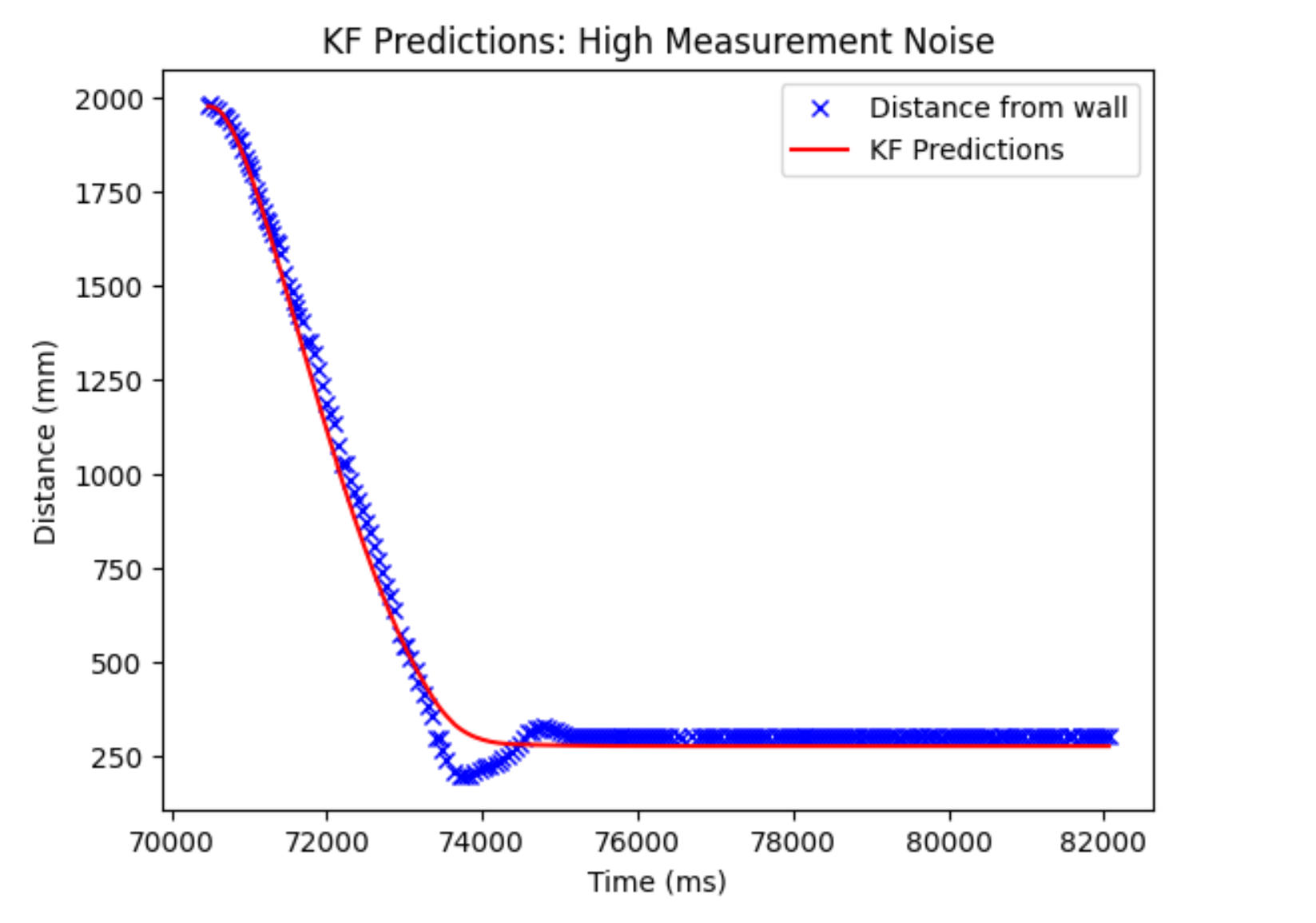
As we can see, the model is still okay, but not the greatest. This could be due to noise or just inconsistencies with the battery.
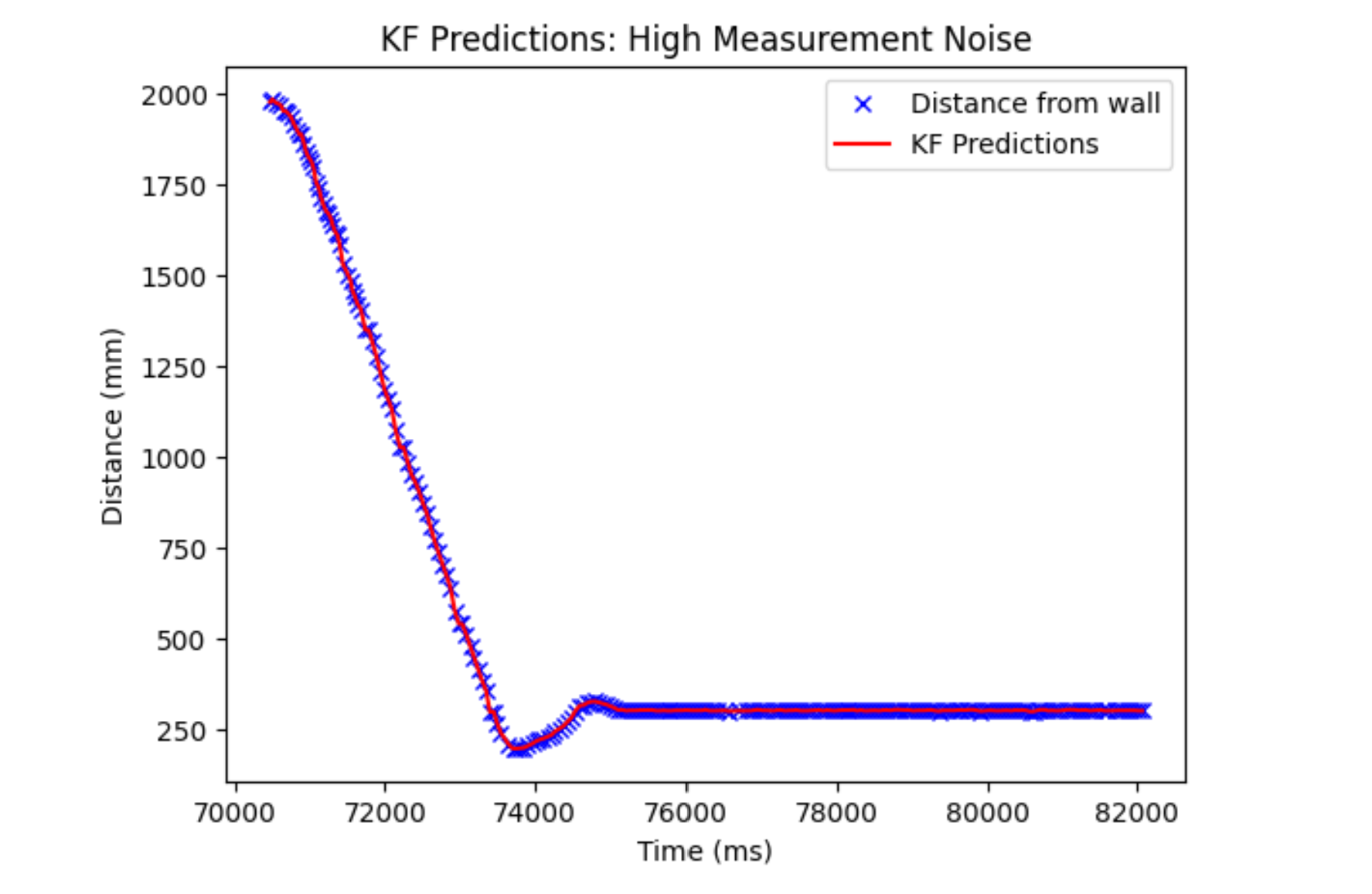
Finally, I switched it so that we only based our prediction off our measurement (turned process noise high and measurement noise low). This looks like it would give us a perfect reading, as we may assume our sensors measure our state. However, this isn’t really helpful to us because we want to use the Kalman filter in order to predict in-between these sensor readings, and our sensors can also be inherently noisy. Thus, if I was running the Kalman filter on board, I would mostly be relying on the prediction steps and then updating that with our sensor values when we get one.
Linear Extrapolator
The Kalman filter worked. However, implementing the linear algebra libraries do not seem fun on the ArduinoIDE and so I used a linear extrapolator in order to predict in between sensor measurements. As long as we’re still getting measurements kind of quick, we can assume a constant linear velocity in between the sensor measurements and it should still work well. A linear extrapolator is also more robust to battery levels and changing floor conditions, as our PID controller assumes that inputting a certain PWM value into our motors will output a certain speed, while our linear extrapolator doesn’t have any of that. However, if our sensor measurements are too slow, then our linear extrapolator will most certainly fail while our Kalman filter can still use its model, which we can see is pretty good, to predict our distance from the wall. Here is the PI control code with the linear extrapolator added:
if(PID_val){
              current_time = millis();
              float dt = (current_time - prev_time)/1000;
              prev_time = current_time; //This value is always updated every loop for interpolation
              //Obtain error

              if(distance < 2000 && change){
                distanceSensor1.setDistanceModeShort();
                change = false;
              }
              if(distanceSensor1.checkForDataReady()){
                distance = distanceSensor1.getDistance();
                float dt_velocity = (current_time - previous_time_dist)/1000;
                velocity = (distance - previous_dist) / dt_velocity;
                previous_time_dist = millis(); //This value is only updated when we get a real sensor measurement
                previous_dist = distance;
                // if(abs(error) < 100){
                //   velocity = 0;
                // }
                distanceSensor1.stopRanging();
                distanceSensor1.startRanging();
              }
              else{
                distance = distance + velocity * dt;
              }
              float error = distance - setpoint;
              float integrated_error = error * dt;
              if(a_error < 20000 || integrated_error < 0){
                a_error = a_error + integrated_error;
              }

              control = kp * error + ki * a_error;
              int speed = abs(control);
              if(control < 0){
                forward = false;
              }
              else{
                forward = true;
              }
              if(speed < 53){
                speed = 53;
              }
              if(speed > 255){
                speed = 255;
              }

              if(abs(error) < 25){
                a_error = 0;
                control = 0;
                velocity = 0;
                stop_robot();
              }
              else if(forward){
                go_foward(speed);
              }
              else{
                go_backwards(speed);
              }

              //Storing data
              if(PID_count < size){
                t[PID_count] = current_time;
                d1s[PID_count] = error;
                d2s[PID_count] = control;
                PID_count++;
              }
            }
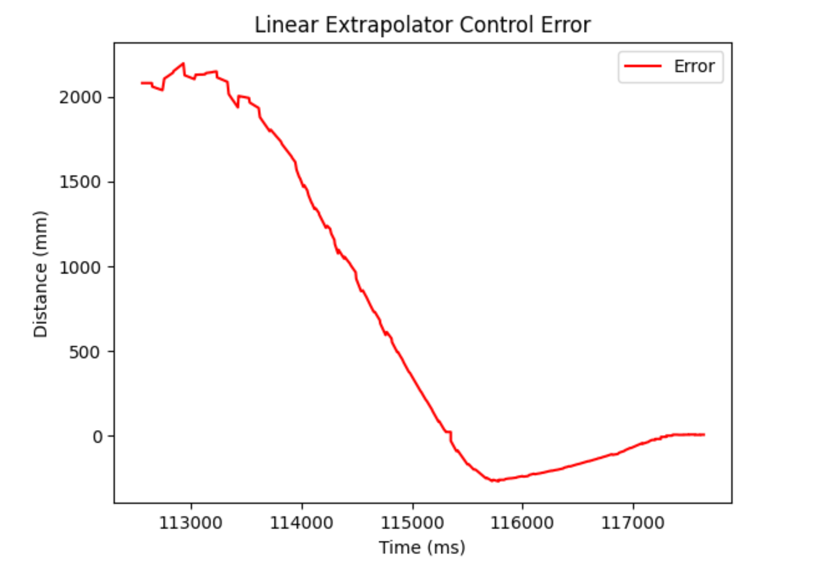
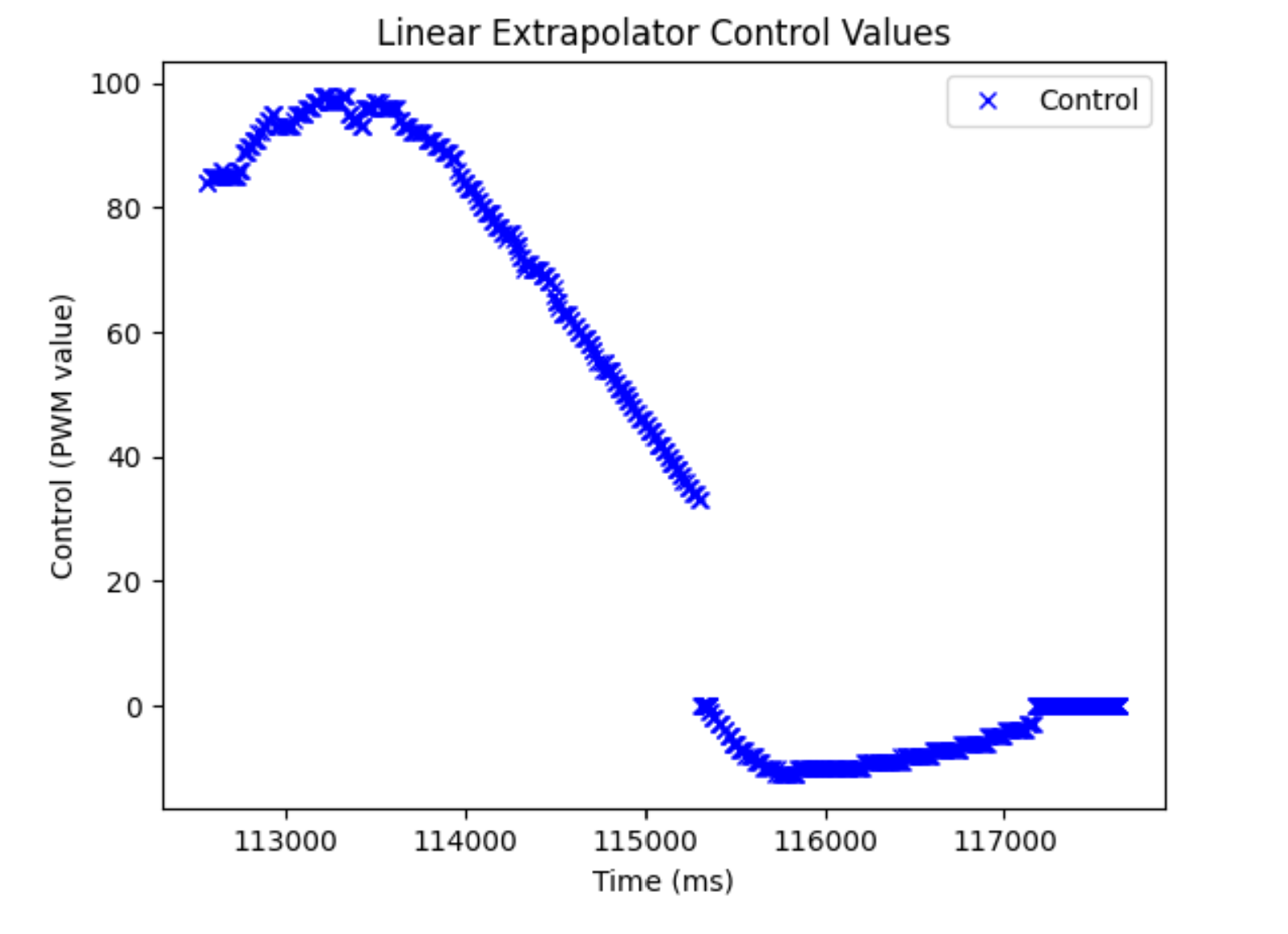
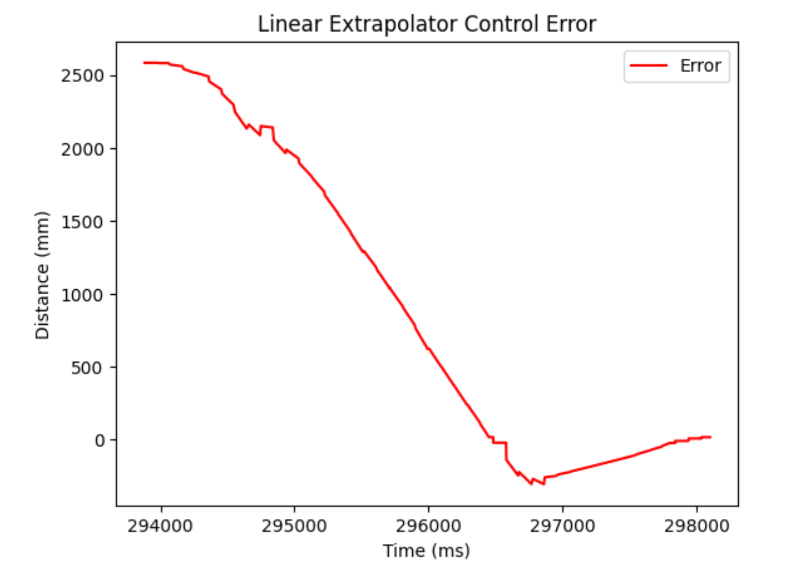
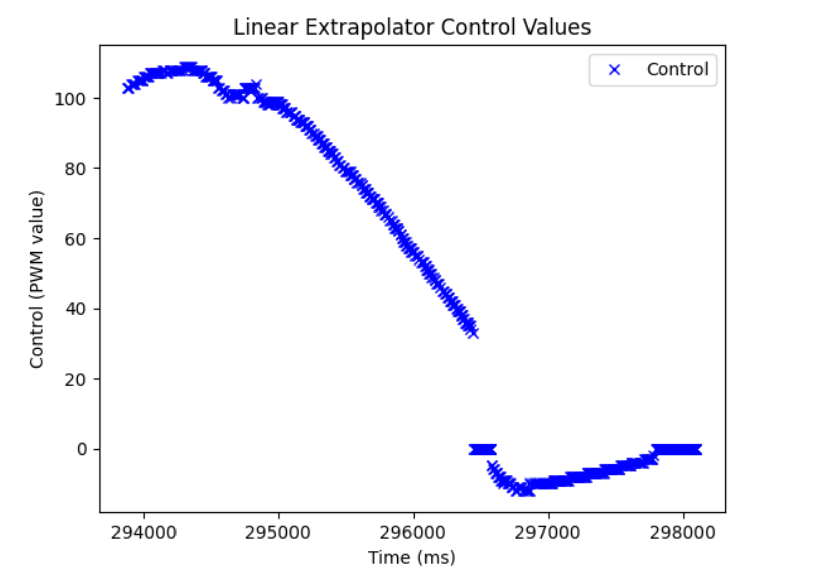
It turned out that our linear extrapolator was almost as our Kalman filter at estimating in between sensor measurements. Here are some plots of my PI controller running with a Kp value of 0.04 and Ki of 0.008. I chose these values because a Kp of 0.05 was too fast when I start further away, so I decided to give some of that power to the Ki value instead of the Kp value.
Here are the plots for that run:
And the video:
I did a run with my old parameters to see the difference and as we can see, it still crashes into the wall. Adding a derivative term would help it not do that.
Plots:
And the video: