Lab 9
The purpose of this lab was to map out a map and learn how to convert points from a robot frame to the global frame.
Building an orientation PID controller
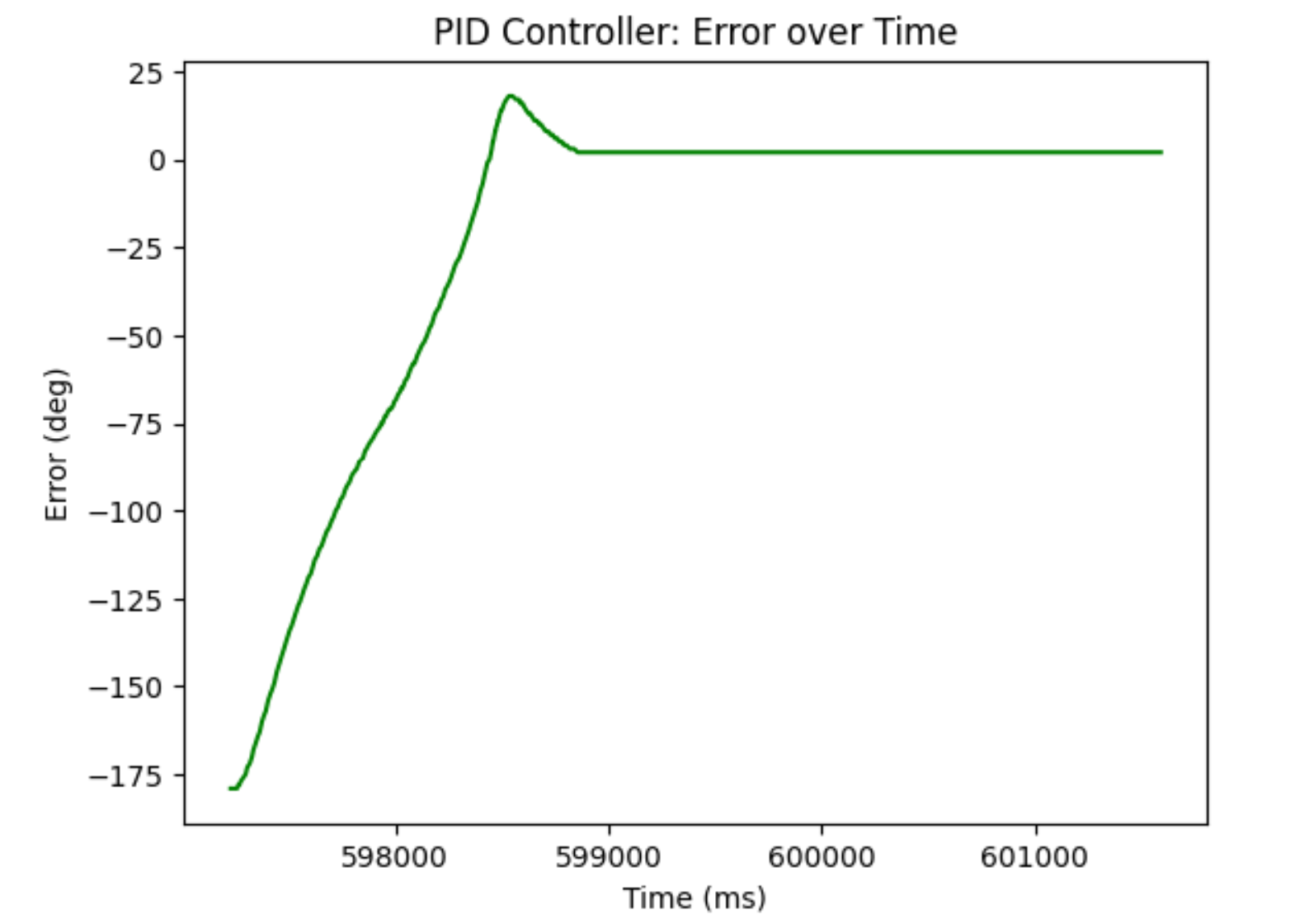
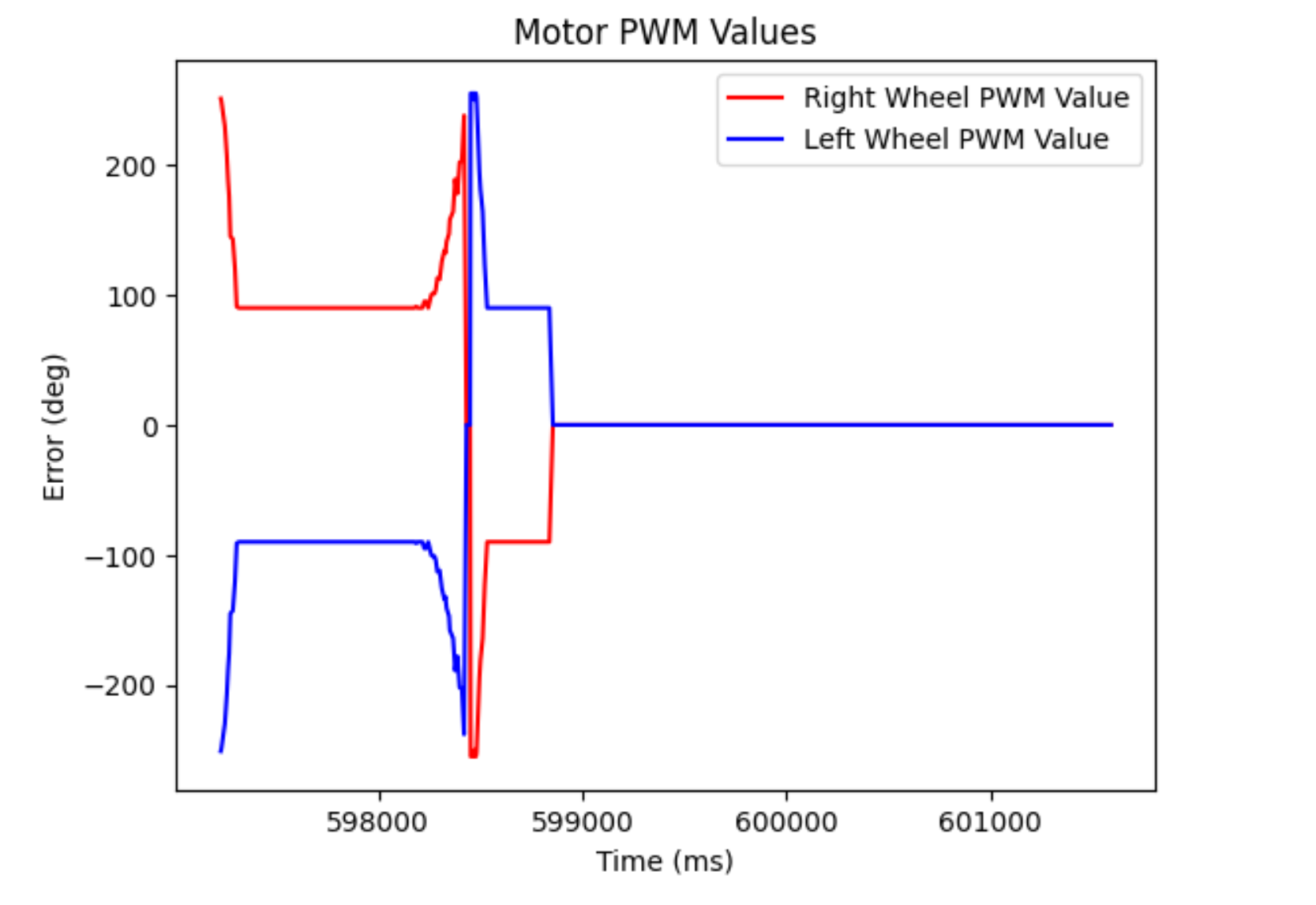
For this lab, I had to build a PID controller to either control orientation or angular speed. I decided to do orientation because I needed it for Lab 8 anyways and it would make taking points at certain angles easier. Because we’re only doing small turns and don’t really need to worry about speed, I essentially made it so that the robot would turn at a fixed speed (that I originally added to overcome deadband), stop at 15 degree increments, and then take a distance measurement. I did have to test my PID controller first. I tested it for a 180 degree turn and took some error values as well as the inputs to the motors. The Kp was 1.4, Ki was 0.1, and Kd was 1. Note that if there is a negative motor input, it means that the motor is turning backwards and I have a function to change the logic for this.
Collecting data
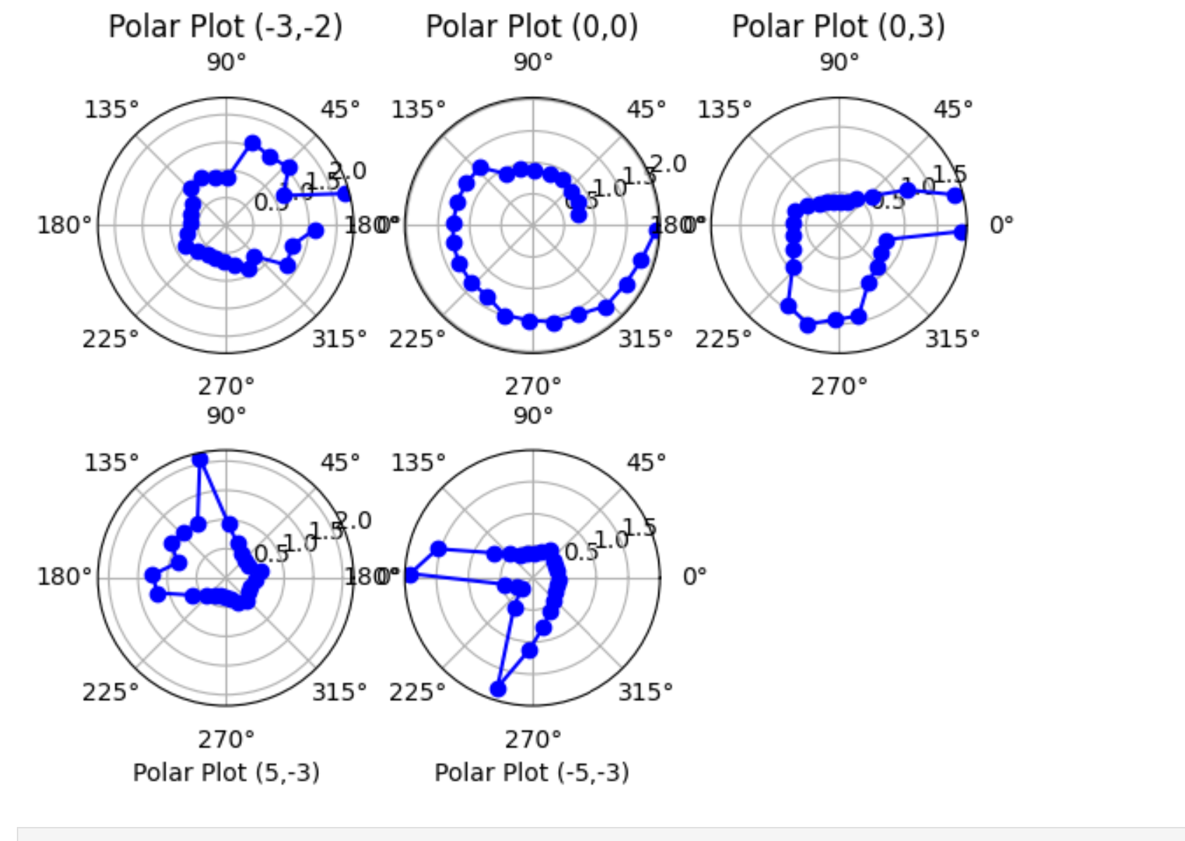
I made the robot stop every 15 degrees for a full 360 degree turn so that it would collect 24 readings. I noticed that there was a tiny bit of overshoot as the robot couldn’t stop on a dime and I made the overcoming deadband a little strong. However, it was able to be fixed by offsetting the values mostly. I also noticed that for some reason, the values were super noisy even when close. The (0,0) values are especially bad, but no matter how many runs I tried, it wouldn’t get much better. Thus, if I were to put my robot in the middle of a 4x4 meter room, I would say that I wouldn’t get very accurate readings. This isn’t because of the PID controller itself, but more because of the noisiness of the ToF sensor at far distances. Thus, we put the robot in different locations in the map and then plot it. If I execute my 360 turn fast enough, drift won’t really matter. I saved all the best datasets into pickle files and plotted them.
Here is a video of my robot collecting values:
And here is a polar plot of all the variables:
Now all I had to was transform these values.
Transformation matrix (not really though)
Because I set my robot so that its angle would match the global angle, I didn’t actually need a transformation matrix to transform my points. If I had, the transformation matrix would have looked like this (\(x_g\) and \(y_g\) are the coordinates of the robot itself in global frame):
\[\begin{bmatrix} cos(\theta) & -sin(\theta) & x_g \\\ sin(\theta) & cos(\theta) & y_g \\\ 0 & 0 & 1 \end{bmatrix}\]However, I could simply convert my distances into global coordinates like so:
\[x = distance * cos(\theta) + x_g\] \[y = distance * sin(\theta) + y_g\]I also had to convert everything into meters (as the points were given to us in feet, which I originally didn’t know and was what was most likely making my transformation matrix not work). I did all of this in a Python notebook.
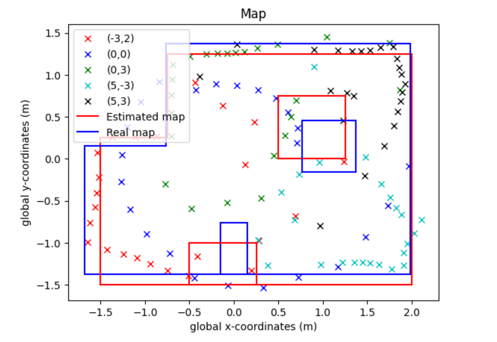
Here is a plot of all my points in global. I mostly ignored my (0,0) readings when trying to figure out where obstacles were. (I still have no clue why my data was so bad from that spot in particular, collected data on 2 different days 3 different times):
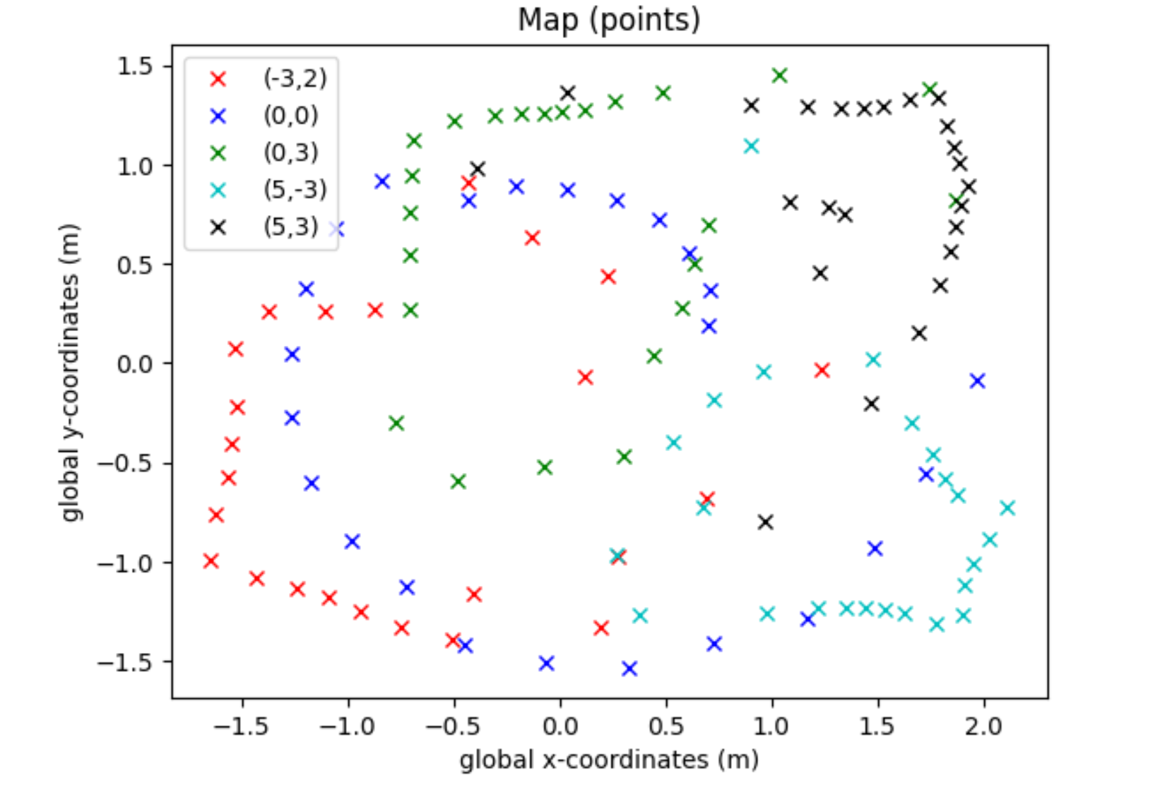
After I got this, I estimated where walls and lines were (mostly ignoring my 0,0 readings).
#Formatted [x1, x2, y1, y2]
wall1 = [-1.5,2,-1.5,-1.5]
wall2 = [2, 2, -1.5, 1.25]
wall3 = [2, -0.75, 1.25, 1.25]
wall4 = [-0.75,-0.75,1.25,.25]
wall5 = [-0.75,-1.5,0.25,0.25]
wall6 = [-1.5,-1.5,-1.5,0.25]

wall7 = [0.5,1.25,0,0]
wall8 = [1.25,1.25,0,0.75]
wall9 = [1.25, 0.5, 0.75, 0.75]
wall10 = [0.5,0.5,0.75,0]

wall11 = [-0.5,-0.5,-1.5,-1]
wall12 = [-0.5,0.25,-1,-1]
wall13 = [0.25,0.25,-1,-1.5]
Here is a plot of that:
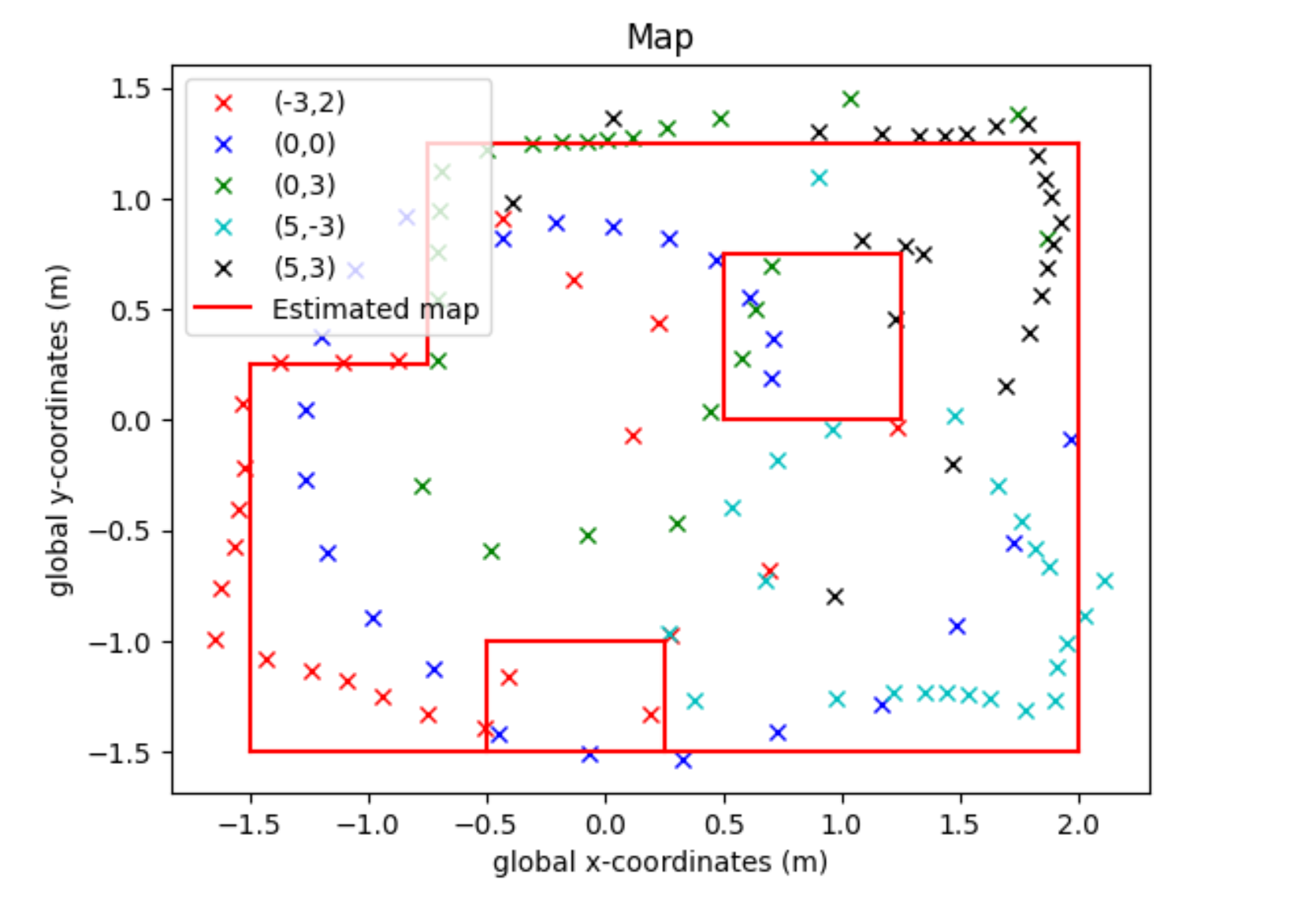
I then compared this to the actual walls that the simulator uses (which this map is based off of). Here are the values (obtained from the simulator)
#Formatted [x1 y1 x2 y2]
r1 = [-1.6764,0.1524,-1.6764,-1.3716]
r2 = [-1.6764,-1.3716,1.9812,-1.3716]
r3 = [1.9812,-1.3716,1.9812,1.3716]
r4 = [1.9812,1.3716,-0.7620,1.3716]
r5 = [-0.7620,1.3716,-0.7620,0.1524]
r6 = [-0.7620,0.1524,-1.6764,0.1524]
r7 = [0.7620,-0.1524,1.3716,-0.1524]
r8 = [1.3716,-0.1524,1.3716,0.4572]
r9 = [1.3716,0.4572,0.7620,0.4572]
r10 = [0.7620,0.4572,0.7620,-0.1524]
r11 = [-0.1524,-1.3716, -0.1524,-0.7620]
r12 = [-0.1524,-0.7620, 0.1524,-0.7620]
r13 = [0.1524,-0.7620,0.1524,-1.3716]
And the plot:
